Advanced Monitor Configuration
Working with Configurations
In most cases monitors can be set up using the monitor manager user interface. This guide is for users that need to set up monitors currently not supported by the UI flow - or those that prefer this method of configuration. There are four ways to build custom monitors using JSON format:
- by accessing a single monitor config
- by accessing the all-monitors config
- via the REST API
- via the Python package whylabs-toolkit Below you will find the details on each of these approaches.
Single-monitor Config Investigator
To inspect the JSON definition of an existing monitor, click on the "View JSON" button that appears on hover in the User Actions column.
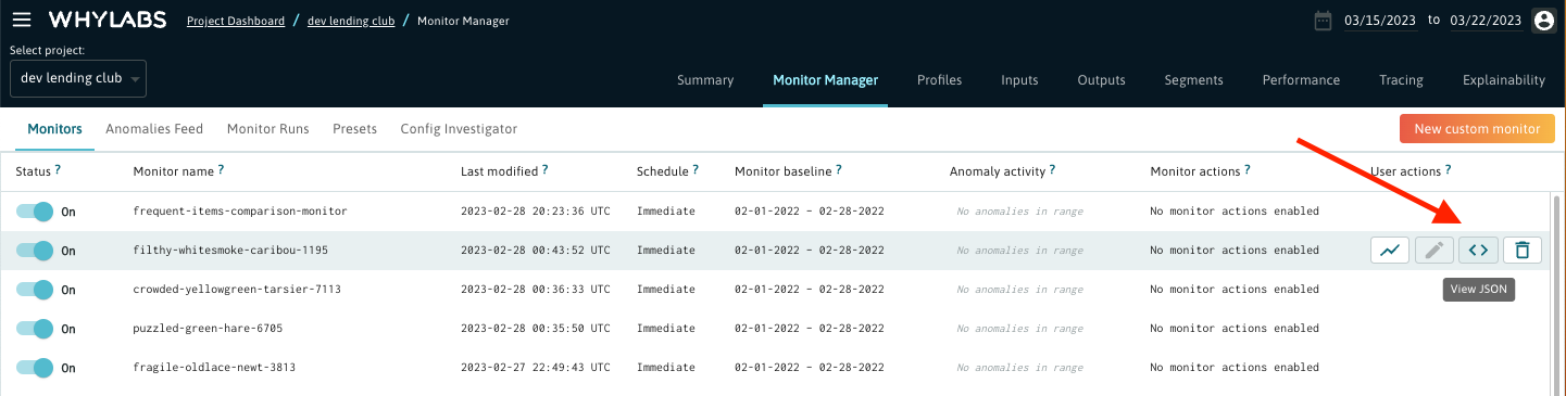
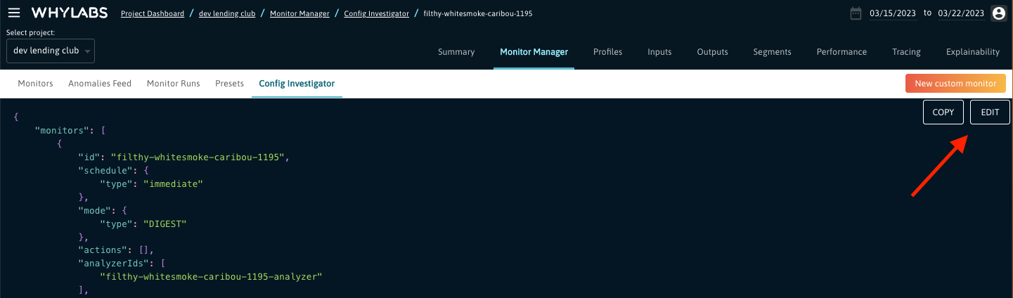
After clicking on it you will see the Config Investigator with a JSON structure consisting of two main elements called "monitors" and "analyzers". For more details on these objects and their role, read this section. To modify this monitor definition, click the "Edit" button that appears when you hover over the JSON content.
Please note that the monitor and analyzer IDs are immutable and cannot be changed.
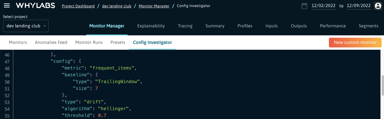
All-monitors Config Investigator
This feature is for advanced users who want to edit the configuration for all of the monitors at once, with minimal guide rails. In order to access it, click on the Config Investigator tab within the Monitor Manager view. Since this feature is currently in beta, contact us to have it enabled for your account.
The JSON configuration that you will see there should have the following structure:
{
    "id": "351bf3cb-705a-4cb8-a727-1839e5052a1a",
    "schemaVersion": 1,
    "orgId": "org-0",
    "datasetId": "model-2130",
    "granularity": "daily",
    "metadata": {...},
    "analyzers": [...],
    "monitors": [...]
}
The "analyzers" and "monitors" keys should contain a list of all analyzer and monitor objects respectively. You can modify this configuration by clicking on the "Edit" button that appears when you hover over the JSON content. Once you entered the edit mode, you can add new monitor and analyzer objects under the respective keys.
REST API
The WhyLabs REST API provides a programmatic way for inspecting and setting up monitors, which can be very helpful if we want to automate the monitor configuration process - for example by applying a set of default monitors to each of our projects. Here are the available APIs:
- GetAnalyzer
- PutAnalyzer
- DeleteAnalyzer
- GetMonitor
- PutMonitor
- DeleteMonitor
- GetMonitorConfigV3
- PutMonitorConfigV3
- PatchMonitorConfigV3
We also provide a Python API client, which enables our users to conveniently use the various APIs.
whylabs-toolkit
Another method for configuring the monitors programmatically is a Python package whylabs-toolkit. It not only facilitates creating new monitors and modifying the existing ones, but also allows various interactions with WhyLabs projects like updating the data schema. For example, the code snippet below shows how to update the trailing window baseline of an existing monitor:
from whylabs_toolkit.monitor import MonitorSetup
from whylabs_toolkit.monitor import MonitorManager

monitor_setup = MonitorSetup(
    monitor_id="my-awesome-monitor"
)
config = monitor_setup.config
config.baseline=TrailingWindowBaseline(size=28)
monitor_setup.config = config

manager = MonitorManager(
    setup=monitor_setup
)
manager.save()
Analyzers vs Monitors
What we generally refer to as a monitor is actually comprised of two elements: an analyzer object and a monitor object. Let us clarify their role and structure.
Once the data profiles computed with whylogs are sent to WhyLabs, they can be analyzed on the platform. This typically means taking a target bucket of time and either comparing it to some baseline data or a fixed threshold. The analyzer is basically defining what kind of analysis will be applied and what data will be covered by it.
While analysis is great, many customers want certain anomalies to alert their internal systems. A monitor specifies which anomalies are of such importance and where to notify (email, PagerDuty, etc).
Let's inspect an example monitor-analyzer pair to understand their structure and dependencies.
{
    "monitors": [
        {
            "schedule": {"type": "immediate"},
            "mode": {"type": "DIGEST"},
            "id": "funny-red-cheetah-2117",
            "displayName": "funny-red-cheetah-2117",
            "analyzerIds": ["funny-red-cheetah-2117-analyzer"],
            "severity": 3,
            "actions": [{
                        "type": "global",
                        "target": "slack"
                      }],
            "metadata": {...}
        }
    ],
    "analyzers": [
        {
            "schedule": {
                "type": "fixed",
                "cadence": "daily"
            },
            "id": "funny-red-cheetah-2117-analyzer",
            "targetMatrix": {
                "type": "column",
                "include": ["group:discrete"],
                "exclude": ["group:output"],
                "segments": []
            },
            "config": {
                "metric": "frequent_items",
                "baseline": {
                    "type": "TrailingWindow",
                    "size": 7
                },
                "type": "drift",
                "algorithm": "hellinger",
                "threshold": 0.7
            },
            "metadata": {...}
        }
    ]
}
The monitor object above has the following elements:
- id - a unique identifier of the monitor object.
- displayName - this is the name of this monitor as shown in the Monitor Manager view. Unlike the ID, the display name can be changed.
- analyzerIds - the list of analyzers that this monitor is triggered by. Currently there is only one analyzer allowed.
- schedule - parameter specifying when to run the monitor job. This monitor is configured to trigger an alert immediately after the analyzer job has finished ("type": "immediate").
- mode - the DIGEST mode means that there will be a single notification message sent containing a summary of all anomalies within the given profile (more details here).
- actions - this parameter lists the so called notification actions, which describe the recipients of the alert messages. In the above example the notifications are sent to a Slack webhook. The main notification channels can be defined in the Notification Settings, which are accessible by admin users for a given organization here.
- severity - indicates the importance of the alerts. This monitor is set to generate alerts with severity equal to 3, which is the default value and indicates the lowest priority. The users can leverage the severity information by setting up rules in their systems receiving the alerts.
Now let's take a closer look at the analyzer object. It consists of 3 main building blocks:
schedule - defining the frequency to run the analyzer, based on UTC time. The job will run at the start of the cadence, so the analyzer in the example will be launched at midnight UTC every day.
targetMatrix - specifies the data covered by the analysis. It allows to target single columns, groups of columns based on their characteristics, entire datasets and specific segments. For more details on constructing the target matrix, see this section
config - the main element describing the type of analysis to be performed. The analyzer above is calculating drift on the frequent items metric (which makes sense since this monitor is applied on discrete features) using Hellinger distance. Drift values above the threshold (set to 0.7 by default) will be marked as anomalies and trigger the related monitor to alert. The baseline will consist of the frequent items from the last 7 days.
For more examples and details of the monitor schema, please check our schema documentation page.
Now having a clearer picture of what analyzers and monitors are, we'll cover their constituents in more detail in the sections below.
Analyzers
Analysis Coverage
Targeting Columns
Whylogs is capable of profiling wide datasets with thousands of columns. Inevitably customers have a subset of columns they wish to focus on for a particular type of analysis. This can be accomplished within the target matrix, which describes the data that should be covered by the given analyzer.
After uploading a profile, each column from a dataset is automatically assigned various attributes, such as input or output, discrete or continuous, and it allows analyzers to be scoped to groups of columns without exhaustively listing names. If schema inference guessed incorrectly or a schema changes, it can be corrected by updating the entity schema editor.
Columns with specific attributes maybe included or excluded from analysys by using one or more of the following options in the targetMatrix:
- group:continuous - Continuous data has an infinite number of possible values that can be measured
- group:discrete - Discrete data is a finite value that can be counted
- group:input - By default columns are considered input unless they contain the word output
- group:output
- * An asterisk wildcard specifies all columns
- sample_column - The name of the column as it was profiled. This is type sensitive
Note: In cases where a column is both included and excluded, it will be excluded.
Example
{
  "targetMatrix": {
    "type": "column",
    "include": [
      "group:discrete",
      "favorite_animal"
    ],
    "exclude": [
      "group:output",
      "sales_engineer_id"
    ]
  }
}
Targeting Segments
whylogs can profile both segmented and unsegmented data. WhyLabs can scope analysis to the overall segment, specific segments, or all segments. This option lives on the targetMatrix config level.
The segments you want to monitor should be defined under the segments key following the format in the example below.
To exclude a specific segment, use the excludeSegments parameter. If a segment is both included and excluded, it will be excluded.
- [] - An empty tags array indicates you would like analysis to run on the overall/entire dataset merged together.
- [{"key" : "purpose", "value": "small_business"}] - Indicates you would like analysis on a specific segment. Note tag keys and values are case sensitive.
- [{"key" : "car_make", "value": "*"}] - Asterisk wildcards are allowed in tag values to in this case generate analysis separately for every car_make in the dataset as well
Example:
"targetMatrix": {
                "include": [
                    "group:discrete"
                ],
                "exclude": [
                    "group:output"
                ],
                "segments": [
                    {
                        "tags": []
                    },
                    {
                        "tags": [
                            {
                                "key": "Store Type",
                                "value": "e-Shop"
                            }
                        ]
                    }
                ],
                "excludeSegments": [
                    {
                        "tags": [
                            {
                                "key": "Store Type",
                                "value": "MBR"
                            }
                        ]
                    }
                ],
                "type": "column"
            }
Targeting Datasets
Some analysis operates at the dataset level rather than on individual columns. This includes monitoring on model accuracy, missing uploads, and more. For example, this analyzer targets the accuracy metric on a classification model.
{
  "id": "cheerful-lemonchiffon-echidna-2235-analyzer",
  "schedule": {
    "type": "fixed",
    "cadence": "daily"
  },
  "targetMatrix": {
    "type": "dataset",
    "segments": []
  },
  "config": {
    "metric": "classification.accuracy",
    "baseline": {
      "type": "TrailingWindow",
      "size": 7
    },
    "type": "diff",
    "mode": "pct",
    "threshold": 2
  }
}
Metrics
WhyLabs provides a wide array of metrics to use for analysis.
Median
Median metric is derived from the KLL datasketch histogram in whylogs. The following analyzer compares a daily target against the previous 14 day trailing window on all columns for both the overall segment and the purpose=small_business segment.
Notes:
factorof 5 is multiplier factor applied to the standard deviation for calculating upper bounds and lower boundsminBatchSizeindicates there must be at least 7 days of data in the 14 days trailing window present in order to analyze. This can be used to make analyzers less noisy when there's not much data in the baseline to compare against. Note thatminBatchSizemust be smaller than the size of the trailing window specified inbaseline.
{
  "id": "my_median_analyzer",
  "schedule": {
    "type": "fixed",
    "cadence": "daily"
  },
  "config": {
    "version": 1,
    "type": "stddev",
    "metric": "median",
    "factor": 5,
    "minBatchSize": 7,
    "baseline": {
      "type": "TrailingWindow",
      "size": 14
    }
  },
  "disabled": false,
  "targetMatrix": {
    "type": "column",
    "include": [
      "*"
    ]
  }
}
Frequent Items
This metric captures the most frequently used values in a dataset. Capturing this metric can be disabled at the whylogs level for customers profiling sensitive data. In this scenario a target's frequent items will be compared against a reference profile with known good data. Since the frequent items metric is only available for discrete features, the targetMatrix is set to group:discrete.
{
  "id": "muddy-green-chinchilla-1108-analyzer",
  "config": {
    "metric": "frequent_items",
    "baseline": {
      "type": "Reference",
      "profileId": "ref-MHxddU9naW0ptlAg"
    },
    "type": "drift",
    "algorithm": "hellinger",
    "threshold": 0.7
  },
  "schedule": {
    "type": "fixed",
    "cadence": "daily"
  },
  "targetMatrix": {
    "type": "column",
    "include": [
      "group:discrete"
    ],
    "exclude": [
      "group:output"
    ]
  }
}
Disabling frequent items collection
To switch off the collection of frequent items, apply the following modification in your whylogs code:
from whylogs.core.schema import DeclarativeSchema
from whylogs.core.metrics import MetricConfig, StandardMetric
from whylogs.core.resolvers import STANDARD_RESOLVER
import whylogs as why

config = MetricConfig(fi_disabled=True)
custom_schema = DeclarativeSchema(STANDARD_RESOLVER, default_config=config)
profile = why.log(pandas=df, schema=custom_schema).profile().view()
Classification Recall
In this scenario the classification recall metric will compare a target against the previous 7 days with an anomaly threshold of two percent change. For more information about sending model performance metrics to WhyLabs see https://nbviewer.org/github/whylabs/whylogs/blob/mainline/python/examples/integrations/writers/Writing_Classification_Performance_Metrics_to_WhyLabs.ipynb
{
  "id": "successful-cornsilk-hamster-3862-analyzer",
  "schedule": {
    "type": "fixed",
    "cadence": "daily"
  },
  "targetMatrix": {
    "type": "dataset",
    "segments": []
  },
  "config": {
    "metric": "classification.recall",
    "baseline": {
      "type": "TrailingWindow",
      "size": 7
    },
    "type": "diff",
    "mode": "pct",
    "threshold": 2
  }
}
Classification Precision
{
  "id": "odd-powderblue-owl-9385-analyzer",
  "schedule": {
    "type": "fixed",
    "cadence": "daily"
  },
  "targetMatrix": {
    "type": "dataset",
    "segments": []
  },
  "config": {
    "metric": "classification.precision",
    "baseline": {
      "type": "TrailingWindow",
      "size": 7
    },
    "type": "diff",
    "mode": "pct",
    "threshold": 2
  }
}
Classification FPR
{
  "id": "odd-powderblue-owl-9385-analyzer",
  "schedule": {
    "type": "fixed",
    "cadence": "daily"
  },
  "targetMatrix": {
    "type": "dataset",
    "segments": []
  },
  "config": {
    "metric": "classification.fpr",
    "baseline": {
      "type": "TrailingWindow",
      "size": 7
    },
    "type": "diff",
    "mode": "pct",
    "threshold": 2
  }
}
Classification Accuracy
{
  "id": "odd-powderblue-owl-9385-analyzer",
  "schedule": {
    "type": "fixed",
    "cadence": "daily"
  },
  "targetMatrix": {
    "type": "dataset",
    "segments": []
  },
  "config": {
    "metric": "classification.accuracy",
    "baseline": {
      "type": "TrailingWindow",
      "size": 7
    },
    "type": "diff",
    "mode": "pct",
    "threshold": 2
  }
}
Classification F1
{
  "id": "odd-powderblue-owl-9385-analyzer",
  "schedule": {
    "type": "fixed",
    "cadence": "daily"
  },
  "targetMatrix": {
    "type": "dataset",
    "segments": []
  },
  "config": {
    "metric": "classification.f1",
    "baseline": {
      "type": "TrailingWindow",
      "size": 7
    },
    "type": "diff",
    "mode": "pct",
    "threshold": 2
  }
}
Regression MSE
{
  "id": "odd-powderblue-owl-9385-analyzer",
  "schedule": {
    "type": "fixed",
    "cadence": "daily"
  },
  "targetMatrix": {
    "type": "dataset",
    "segments": []
  },
  "config": {
    "metric": "regression.mse",
    "baseline": {
      "type": "TrailingWindow",
      "size": 7
    },
    "type": "diff",
    "mode": "pct",
    "threshold": 2
  }
}
Regression MAE
{
  "id": "odd-powderblue-owl-9385-analyzer",
  "schedule": {
    "type": "fixed",
    "cadence": "daily"
  },
  "targetMatrix": {
    "type": "dataset",
    "segments": []
  },
  "config": {
    "metric": "regression.mae",
    "baseline": {
      "type": "TrailingWindow",
      "size": 7
    },
    "type": "diff",
    "mode": "pct",
    "threshold": 2
  }
}
Regression RMSE
{
  "id": "odd-powderblue-owl-9385-analyzer",
  "schedule": {
    "type": "fixed",
    "cadence": "daily"
  },
  "targetMatrix": {
    "type": "dataset",
    "segments": []
  },
  "config": {
    "metric": "regression.rmse",
    "baseline": {
      "type": "TrailingWindow",
      "size": 7
    },
    "type": "diff",
    "mode": "pct",
    "threshold": 2
  }
}
Uniqueness
Uniqueness in whylogs is efficiently measured with the HyperLogLog algorithm with typically %2 margin of error.
- unique_est - The estimated unique values
- unique_est_ratio - estimated unique/total count
{
  "id": "pleasant-linen-albatross-6992-analyzer",
  "schedule": {
    "type": "fixed",
    "cadence": "daily"
  },
  "targetMatrix": {
    "type": "column",
    "include": [
      "group:discrete"
    ],
    "exclude": [
      "group:output"
    ],
    "segments": []
  },
  "config": {
    "metric": "unique_est_ratio",
    "type": "fixed",
    "upper": 0.5,
    "lower": 0.2
  }
}
Count
{
  "id": "pleasant-linen-albatross-6992-analyzer",
  "schedule": {
    "type": "fixed",
    "cadence": "daily"
  },
  "targetMatrix": {
    "type": "column",
    "include": [
      "group:continuous"
    ],
    "exclude": [
      "group:output"
    ],
    "segments": []
  },
  "config": {
    "metric": "count",
    "type": "fixed",
    "upper": 100,
    "lower": 10
  }
}
Mean
{
  "id": "pleasant-linen-albatross-6992-analyzer",
  "schedule": {
    "type": "fixed",
    "cadence": "daily"
  },
  "targetMatrix": {
    "type": "column",
    "include": [
      "group:continuous"
    ],
    "exclude": [
      "group:output"
    ],
    "segments": []
  },
  "config": {
    "metric": "mean",
    "type": "fixed",
    "lower": 10.0
  }
}
Min/Max
Min and max values are derived from the kll sketch.
{
  "id": "pleasant-linen-albatross-6992-analyzer",
  "schedule": {
    "type": "fixed",
    "cadence": "daily"
  },
  "targetMatrix": {
    "type": "column",
    "include": [
      "group:continuous"
    ],
    "exclude": [
      "group:output"
    ],
    "segments": []
  },
  "config": {
    "metric": "min",
    "type": "fixed",
    "lower": 10.0
  }
}
Schema Count Metrics
Whylogs performs schema inference, tracking counts for inferred data types. Each count as well as a ratio of that count divided by the total can be accessed with the following metrics:
- count_bool
- count_bool_ratio
- count_integral
- count_integral_ratio
- count_fractional
- count_fractional_ratio
- count_string
- count_string_ratio
- count_null
- count_null_ratio
{
  "id": "pleasant-linen-albatross-6992-analyzer",
  "schedule": {
    "type": "fixed",
    "cadence": "daily"
  },
  "targetMatrix": {
    "type": "column",
    "include": [
      "group:continuous"
    ],
    "exclude": [
      "group:output"
    ],
    "segments": []
  },
  "config": {
    "metric": "count_bool",
    "type": "fixed",
    "lower": 10
  }
}
Missing Data
Most metrics await profile data to be uploaded before analyzing however missingDatapoint is an exception. This metric is most useful for detecting broken integrations with WhyLabs. Use dataReadinessDuration to control how long to wait before notifying. While very similar in purpose to the secondsSinceLastUpload metric, the missingDatapoint analyzer can detect misconfigured timestamps at the whylogs level. Note this metric does not fire for datasets which have never had data uploaded.
In the following scenario this analyzer will create an anomaly for a datapoint which has not been uploaded to WhyLabs after 1 day and 18 hours has passed. Given the empty tags array it will create an anomaly if no data has been uploaded for the entire dataset. Segmentation can be used to raise alarms for specific segments. See "Targeting Segments" for more information.
{
  "id": "missing-datapoint-analyzer",
  "schedule": {
    "type": "fixed",
    "cadence": "daily"
  },
  "disabled": false,
  "targetMatrix": {
    "type": "dataset",
    "segments": []
  },
  "dataReadinessDuration": "P1DT18H",
  "config": {
    "metric": "missingDatapoint",
    "type": "fixed",
    "upper": 0
  }
}
Detecting Missing Data per Segment
In the example below a dataset has been segmented by country. We wish to alert if any countries stopped receiving data after 18 hours has passed.
{
  "id": "missing-datapoint-analyzer",
  "schedule": {
    "type": "fixed",
    "cadence": "daily"
  },
  "disabled": false,
  "targetMatrix": {
    "type": "dataset",
    "segments": [
      {
        "tags": [
          {
            "key": "country",
            "value": "*"
          }
        ]
      }
    ]
  },
  "dataReadinessDuration": "PT18H",
  "backfillGracePeriodDuration": "P30D",
  "config": {
    "metric": "missingDatapoint",
    "type": "fixed",
    "upper": 0
  }
}
Seconds Since Last Upload
Most metrics await profile data to be uploaded before analyzing however secondsSinceLastUpload is an exception. In this scenario an anomaly will be generated when it's been more than a day since the last upload for this dataset. Note this metric does not fire for datasets which have never had data uploaded.
{
  "id": "missing_upload_analyzer",
  "schedule": {
    "type": "fixed",
    "cadence": "daily"
  },
  "config": {
    "type": "fixed",
    "version": 1,
    "metric": "secondsSinceLastUpload",
    "upper": 86400
  },
  "disabled": false,
  "targetMatrix": {
    "type": "dataset",
    "segments": []
  }
}
Analysis types
WhyLabs provides a number of ways to compare targets to baseline data.
Drift
WhyLabs uses Hellinger distance to calculate drift. WhyLabs uses Hellinger distance because it is a symmetric (unlike say, KL divergence), well defined for categorical and numerical features (unlike say, Kolmogorov-Smirnov statistic), and has a clear analogy to Euclidean distance. It's not as popular in the ML community, but has a stronger adoption in both statistics and physics. If additional drift algorithms are needed, contact us.
{
  "id": "muddy-green-chinchilla-1108-analyzer",
  "config": {
    "metric": "frequent_items",
    "baseline": {
      "type": "Reference",
      "profileId": "ref-MHxddU9naW0ptlAg"
    },
    "type": "drift",
    "algorithm": "hellinger",
    "threshold": 0.7
  },
  "schedule": {
    "type": "fixed",
    "cadence": "daily"
  },
  "targetMatrix": {
    "type": "column",
    "include": [
      "group:discrete"
    ],
    "exclude": [
      "group:output"
    ]
  }
}
Click here to see this monitor's schema documentation.
Diff
A target can be compared to a baseline with the difference expressed as either a percentage ("mode": "pct") or an absolute value ("mode": "abs"). In this case an anomaly would be generated for a 50% increase.
If we need our monitor to alert in case of a bidirectional changes (both for an increase as well as a decrease), we need to remove the thresholdType parameter.
{
  "id": "cheerful-lemonchiffon-echidna-4053-analyzer",
  "config": {
    "metric": "classification.accuracy",
    "type": "diff",
    "mode": "pct",
    "threshold": 50,
    "thresholdType": "upper",
    "baseline": {
      "type": "TrailingWindow",
      "size": 7
    }
  },
  "schedule": {
    "type": "fixed",
    "cadence": "daily"
  },
  "targetMatrix": {
    "type": "dataset",
    "segments": []
  }
}
Click here to see this monitor's schema documentation.
Fixed Threshold
Compare a target against a static upper/lower bound. It can be uni-directional (i.e. have only one threshold specified).
An example use case for this monitor type would be to alert in case of negative values - we would need to apply a lower threshold of 0 to the min value metric as in the example below:
{
  "id": "fixed-threshold-analyzer",
  "config": {
    "metric": "min",
    "type": "fixed",
    "lower": 0
  },
  "schedule": {
    "type": "fixed",
    "cadence": "daily"
  },
  "disabled": false,
  "targetMatrix": {
    "type": "column",
    "include": "group:continuous"
    "segments": [
      {
        "tags": []
      }
    ]
  }
}
Click here to see this monitor's schema documentation.
Standard Deviations
Classic outlier detection approach applicable to numerical data. Calculates upper bounds and lower bounds based on stddev from a series of numbers.
factor is a multiplier applied to the standard deviation for calculating upper bounds and lower bounds. If unspecified, factor defaults to 3.
Click here to see this monitor's schema documentation.
{
  "id": "my_analyzer",
  "schedule": {
    "type": "fixed",
    "cadence": "daily"
  },
  "config": {
    "type": "stddev",
    "factor": 5,
    "metric": "median",
    "minBatchSize": 7,
    "baseline": {
      "type": "TrailingWindow",
      "size": 14
    }
  },
  "disabled": false,
  "targetMatrix": {
    "type": "column",
    "include": [
      "*"
    ]
  }
}
By default the stddev analyzer will generate an alert when the targeted metric
value either exceeds the calculated upper-bound or falls below the calculated
lower-bound. You can turn this into a single-sided analyzer by adding
thresholdType to the config. thresholdType can take on two values, "upper"
or "lower", indicating which limit should be used for deciding if an alert is
generated.
  "config": {
    "type": "stddev",
    "factor": 5,
    "metric": "median",
    "thresholdType": "upper",
    "minBatchSize": 7,
    "baseline": {
      "type": "TrailingWindow",
      "size": 14
    }
Example results of single-sided upper threshold stddev analyzer.
Static Thresholds
Stddev is one of our more versatile analyzers. In addition to the calculated
thresholds, stddev analyzer can be constrained by optional static
thresholds, minLowerThreshold and maxUpperThreshold. By default a stddev
analyzer will alert if the target value exceeds the calculated upper-bound, or
if the target value exceeds the static maxUpperThreshold, if supplied. An
alert will also be generated if the target value falls below the calculated
lower-bound or below minLowerThreshold.
  "config": {
      "baseline": {
          "size": 7,
          "type": "TrailingWindow"
      },
      "factor": 1.96,
      "metric": "unique_est_ratio",
      "type": "stddev",
      "maxUpperThreshold": 0.022,
      "minLowerThreshold": 0.013
  },
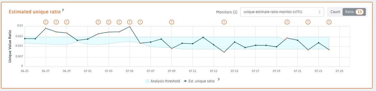
Example results of stddev analyzer with static thresholds.
Some metrics, like "count_null_ratio" or "unique_est_ratio" with high count
denominators, can be extremely small, e.g unique_est_ratio=10-6 is
not unusual. A baseline of extremely small ratios will generate a very small
mean and even smaller stddev. Any deviation from baseline is likely to exceed
any reasonable factor of the stddev, leading to frequent spurious alerts.
maxUpperThreshold does not help because it is usually an alternative to the
calculated threshold, not a constraint to dampen alerts.
However the limitType property can change the interpretation of the static
thresholds and help dampen spurious alerts. By setting
limitType to "and", the analyzer will generate an alert only if the target
values exceeds the calculated threhold, AND it exceeds maxUpperThreshold.
In this way maxUpperThreshold becomes a constraint on alerting, resulting in
less noisy monitors.
    "config": {
        "baseline": {
            "size": 7,
            "type": "TrailingWindow"
        },
        "factor": 1.96,
        "metric": "unique_est_ratio",
        "type": "stddev",
        "maxUpperThreshold": 0.022,
        "minLowerThreshold": 0.013,
        "limitType": "and"
    },
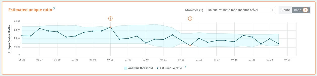
Example results of stddev analyzer with static thresholds and limitType "and".
Seasonal Monitor
Example seasonal monitor configuration (only the analyzer object part):
    {
    "analyzers": [
        {
            "id": "sarima-analyzer",
            "tags": [],
            "schedule": {
                "type": "fixed",
                "cadence": "daily"
            },
            "targetMatrix": {
                "segments": [],
                "type": "column",
                "include": [
                    "*"
                ]
            },
            "config": {
                "metric": "median",
                "type": "seasonal",
                "algorithm": "arima",
                "minBatchSize": 30,
                "alpha": 0.05,
                "baseline": {
                    "type": "TrailingWindow",
                    "size": 90
                },
                "stddevTimeRanges": [
                    {
                        "end": "2024-01-02T00:00:00+00:00",
                        "start": "2023-11-21T00:00:00+00:00"
                    }
                ],
                "stddevFactor": 3
            }
        }
    ]
}
Click here to see this monitor's schema documentation.
SARIMA overview
The SARIMA acronym stands for Seasonal Auto-Regressive Integrated Moving Average. SARIMA is a time-series forecasting model which combines properties from several different forecasting techniques.
The concepts behind SARIMA can be summarized as:
- Seasonal - Predictions are influenced by previous values and prediction errors which are offset by some number of seasonal cycles.
- Auto-Regressive - Predictions are influenced by some configurable number of previous values immediately preceding the prediction.
- Integrated - A differencing technique is performed some configurable number of times to arrive at an approximately stationary series (constant mean and variance) which can be more easily analyzed.
- Moving Average - Predictions are influenced by the errors associated with some configurable number of previous predictions.
The SARIMA model takes the form of a linear expression with contributions from previous values in the series as well as contributions from prediction errors from previous timesteps.
This linear function is trained on some time series which has been transformed to be approximately stationary (constant mean and variance). This training process involves tuning the coefficients from this linear expression such that the squared error is minimized.
SARIMA parameters
The form of this linear expression is determined by 7 hyper-parameters, commonly expressed as SARIMA(p,d,q)(P,D,Q)s.
Our SARIMA implementation uses the following hyperparameters:
Order (p, d, q)
p = 1 d = 0 q = 0
Seasonal order (P,D,Q)s
P = 2 D = 1 Q = 0 s = 7
The prediction errors of the trained model form a distribution which is used to calculate a 95% confidence interval surrounding the model’s prediction. WhyLabs utilizes this 95% confidence interval for anomaly detection and raises an alert for any observed values which fall outside of this confidence interval. The monitor configuration has a parameter alpha, which can be used to control this confidence interval. By default alpha is set to 0.05, which means that the algorithm will calculate a 95% confidence interval around predictions. The lower alpha is, the more narrow the confidence interval gets, which in turn leads to a more strict anomaly detection process.
Post-processing: clamping logic
The calculation clamps the CI bounds to the standard deviation over all values in the baseline (including dates within stddevTimeRanges). The width of the clamping function is controlled by stddevFactor in the analyzer config. This is done for every date, regardless of the contents of stddevTimeRanges. The code below illustrates the clamping procedure. The variables lower and upper are denoting confidence interval bounds generated with the seasonal ARIMA algorithm.
 lower_std = forecast - stddev * stddevFactor
 upper_std = forecast + stddev * stddevFactor
 if lower < lower_std:
     lower = lower_std
 if upper > upper_std:
     upper = upper_std
Anomaly handling in SARIMA
Our SARIMA implementation includes an anomaly handling logic. The idea is to replace anomalies so they do not throw off baseline calculations in the future. Anomalies are replaced in future baselines with a random value chosen from within the 95% CI (confidence interval) of the forecast. This means that in some cases the anomalous value is substituted by a value that is 95% likely to be equal to the metric for which the forecast is executed. The probability of replacing an anomaly is by default 50%. Within the stddevTimeRanges intervals that probability goes up to 80/20 in favor of replacement.
Handling annual periods with expected anomalous behavior
In order to accommodate for annual periods of increased data volatility (e.g. Black Friday sale, holiday season, etc.), we introduced a stddevTimeRanges parameter that allows the user to specify a list of such time periods. The specified time ranges are excluded from the baseline and they also have an increased probability of anomaly replacement (from 50% to 80%).
Below you can see an example value for the stddevTimeRanges parameter:
"stddevTimeRanges": [
      { "start": "2022-11-05T00:00:00+00:00", "end": "2022-11-15T00:00:00+00:00" }
    ]
Expected Values Comparison
Compare a numeric metric against a static set of values. In the example below the count_bool metric is expected to be either 0 or 10. A value of 7 would generate an anomaly.
Operators
- in - Metric is expected to be contained within these values, generate an anomaly otherwise
- not_in - Metric is expected to never fall within these values, generate an anomaly if they do
Expected
- int - Compare two integers
- float - Compare two floating point numbers down to the unit of the least precision
{
  "id": "list-comparison-6992-analyzer",
  "schedule": {
    "type": "fixed",
    "cadence": "daily"
  },
  "targetMatrix": {
    "type": "column",
    "include": [
      "*"
    ],
    "segments": []
  },
  "config": {
    "metric": "count_bool",
    "type": "list_comparison",
    "operator": "in",
    "expected": [
      {"int": 0},
      {"int": 10}
    ]
  }
}
Frequent String Comparison
The frequent string analyzer utilizes the frequent item sketch. Capturing this can be disabled at the whylogs level for customers profiling sensitive data. In the example below a reference profile with the column dayOfWeek has been uploaded with Monday-Sunday as expected values. A target value of "September" would generate an anomaly.
Note: This analyzer is only suitable for low cardinality (<100 possible value) columns. Comparisons are case-sensitive. In later versions of whylogs, only the first 128 characters of a string are considered significant.
Operators
- eq - Target is expected to contain every element in the baseline and vice versa. When not the case, generate an anomaly.
- target_includes_all_baseline - Target is expected to contain every element in the baseline. When not the case, generate an anomaly.
- baseline_includes_all_target - Baseline is expected to contain every element in the target. When not the case, generate an anomaly.
{
  "id": "frequent-items-comparison-analyzer",
  "schedule": {
    "type": "fixed",
    "cadence": "daily"
  },
  "targetMatrix": {
    "type": "column",
    "include": [
      "dayOfWeek"
    ],
    "segments": []
  },
  "config": {
    "metric": "frequent_items",
    "type": "frequent_string_comparison",
    "operator": "baseline_includes_all_target",
    "baseline": {
      "type": "Reference",
      "profileId": "ref-MHxddU9naW0ptlAg"
    }
  }
}
Monotonic Analysis
The monotonic analyzer is used for detecting a metric has increased or decreased between sequential target buckets. In the analyzer below, the sales column must always be increasing and would generate an anomaly if sales dropped from one day to the next.
- targetSize: How many sequential buckets are to be evaluated together
- numBuckets: Out of the target size how many instances of the specified direction are required to be considered an anomaly
- direction: INCREASING/DECREASING, specifies which direction is considered anomalous
{
            "id": "excited-rosybrown-elephant-8028-analyzer",
            "targetSize": 2,
            "schedule": {
                "type": "fixed",
                "cadence": "daily"
            },
            "config": {
                "type": "monotonic",
                "metric": "count",
                "direction": "DECREASING",
                "numBuckets": 1
            },
            "disabled": false,
            "targetMatrix": {
                "type": "column",
                "include": [
                    "sales"
                ]
            }
        }
Setting the Baseline
Trailing Windows
The most frequently used baseline would be the trailing window. Use the size parameter to indicate how much baseline to use for comparison. This aligns with the dataset granularity, so a baseline of 7 on a daily model would use 7 days worth of data as the baseline. Many metrics can be configured with a minBatchSize to prevent analysis when there's insufficient baseline. This is useful for making alerts on sparse data less chatty.
{
  "id": "cheerful-lemonchiffon-2244-analyzer",
  "schedule": {
    "type": "fixed",
    "cadence": "daily"
  },
  "targetMatrix": {
    "type": "dataset",
    "segments": []
  },
  "config": {
    "metric": "classification.accuracy",
    "baseline": {
      "type": "TrailingWindow",
      "size": 7
    },
    "type": "diff",
    "mode": "pct",
    "threshold": 2
  }
}
Exclusion Ranges
Trailing window baselines can exclude time ranges. In this scenario the first day of January is excluded from being part of a baseline.
{
  "id": "successful-cornsilk-hamster-3862-analyzer",
  "config": {
    "metric": "classification.recall",
    "baseline": {
      "type": "TrailingWindow",
      "size": 7,
      "exclusionRanges": [
        {
          "start": "2021-01-01T00:00:00.000Z",
          "end": "2021-01-02T00:00:00.000Z"
        }
      ]
    },
    "type": "diff",
    "mode": "pct",
    "threshold": 2
  },
  "schedule": {
    "type": "fixed",
    "cadence": "daily"
  },
  "targetMatrix": {
    "type": "dataset",
    "segments": []
  }
}
Baseline Exclusion Schedules
In cases where a baseline should exclude dates on a recurring basis, setting exclusionRanges as list of fixed time ranges would be cumbersome. To achieve such an exclusion, add a cron expression to config.baseline.exclusionSchedule defining the schedule for exclusion. Note this feature is currently only available for TrailingWindow baseline configs.
Some Examples:
- 0 0 25 12 * Exclude December 25th from baseline
- 0 0 * * 1-5 Exclude Monday-Friday from baseline
- 0 0 * * 6,0 Exclude Weekends from baseline
- 0 9-17 * * * Exclude hours 9-17 (hourly models only) from baseline
In the example below we have a 7d trailing window baseline which excludes the weekends:
{
  "id": "odd-azure-lyrebird-799-analyzer",
  "config": {
    "baseline": {
      "size": 7,
      "type": "TrailingWindow",
      "exclusionSchedule": {
        "cron": "0 0 * * 6,0",
        "type": "cron"
      }
    }
  }
}
Reference Profiles
Instead of comparing targets to some variation on a rolling time window baseline, reference profiles are referenced by profileId. This scenario compares a target every day against a profile of known good data for drift on frequent items. For more information about sending reference profiles to whylabs see whylogs documentation.
{
  "id": "muddy-green-chinchilla-1108-analyzer",
  "config": {
    "metric": "frequent_items",
    "baseline": {
      "type": "Reference",
      "profileId": "ref-MHxddU9naW0ptlAg"
    },
    "type": "drift",
    "algorithm": "hellinger",
    "threshold": 0.7
  },
  "schedule": {
    "type": "fixed",
    "cadence": "daily"
  },
  "targetMatrix": {
    "type": "column",
    "include": [
      "group:discrete"
    ],
    "exclude": [
      "group:output"
    ]
  }
}
Fixed Time Range
Time range baselines compare a target against a baseline with a fixed start/end time range. This scenario performs drift detection on the histogram comparing a target against a fixed period of time which was considered normal.
{
  "id": "continuous-distribution-58f73412",
  "config": {
    "baseline": {
      "type": "TimeRange",
      "range": {
        "start": "2022-02-25T00:00:000Z",
        "end": "2022-03-25T00:00:000Z"
      }
    },
    "metric": "histogram",
    "type": "drift",
    "algorithm": "hellinger",
    "threshold": 0.7,
    "minBatchSize": 1
  },
  "schedule": {
    "type": "fixed",
    "cadence": "daily"
  },
  "disabled": false,
  "targetMatrix": {
    "type": "column",
    "include": [
      "group:continuous"
    ]
  },
  "backfillGracePeriodDuration": "P30D"
}
Scheduling Analysis
WhyLabs provides a number of configuration options giving you full control over exactly when analysis and monitoring runs.
Dataset Granularity
When creating models you're asked to provide a dataset granularity which determines the analysis granularity and to a large extent the analysis cadence. WhyLabs currently supports four options:
Hourly
Hourly datasets are sometimes used in profiling streaming applications. Data can be profiled with any timestamp and the UI will automatically roll up data to hourly granularity. When analyzing, a single target hour will be compared to the configured baseline.
The default flow waits for the hour to end before beginning analysis, assuming more data could arrive. For example, data logged with timestamps of [1:03, 1:35] to wait until after the hour has ended (2pm) before beginning analysis.
Daily
Daily datasets conclude at midnight UTC. When analyzing, a single target day will be compared to the configured baseline.
The default flow waits for the day to end before beginning analysis, assuming more data could arrive. If that's too long of a wait and more eager analysis is desired, read the section below on allowPartialTargetBatches.
Weekly
Weekly datasets conclude on Monday at midnight UTC. When analyzing, a single target week will be compared to the configured baseline.
The default flow waits for the week to end before beginning analysis, assuming more data could arrive. If that's too long of a wait and more eager analysis is desired, read the section below on allowPartialTargetBatches.
Monthly
Monthly datasets conclude on 1st of each month at midnight UTC. When analyzing, a single target month will be compared to the configured baseline.
The default flow waits for the month to end before beginning analysis, assuming more data could arrive. If that's too long of a wait and more eager analysis is desired, read the section below on allowPartialTargetBatches.
Gating Analysis
Some data pipelines run on a fixed schedule, some run when cloud resources are cheaper, some run continuously in a distributed environment, and sometimes they're just running on a laptop.
WhyLabs provides a number of gating options to hold off on analysis until you're done profiling a hour/day/week/month. Analysis is immutable unless explicitly deleted, so controlling when analyzers run avoids running analysis when more data is expected to arrive.
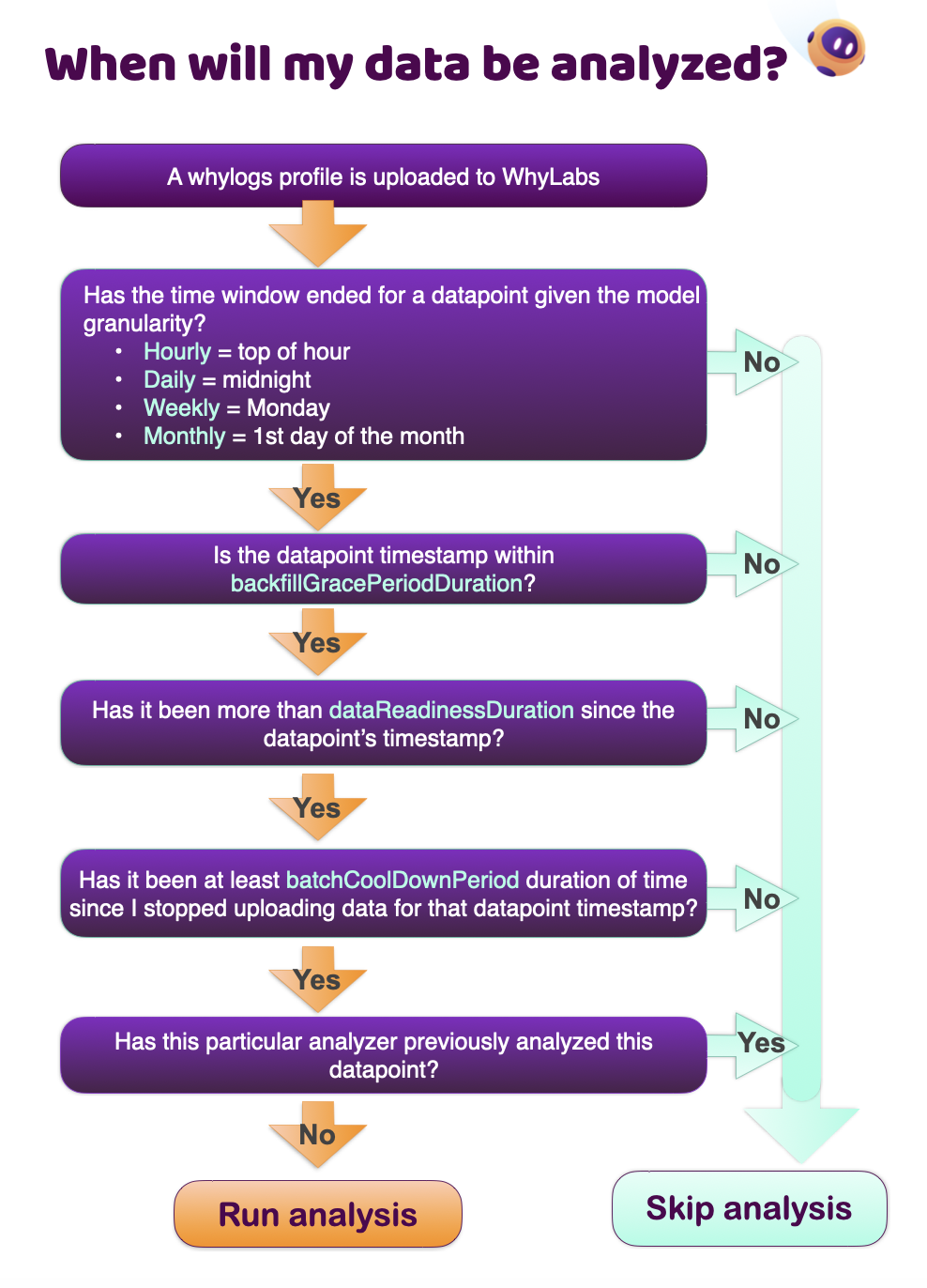
Data Readiness Duration
If you need to delay the analysis, optionally specify a dataReadinessDuration at the analyzer configuration level. If you recall from dataset granularities, a dataset marked as daily would normally be considered ready for analysis at midnight UTC next next day. A common scenario would be a customer running their data pipeline later in the day and wanting to postpone analysis a minimum fixed amount of time to accommodate. This is a perfect case for applying the dataReadinessDuration parameter.
It's important to note that the clock starts at the batch timestamp, which for daily models is midnight UTC. For example a batch holding all data from October 1st 2023 will have a timestamp of 2023-10-01 00:00:00.000.
The default dataReadinessDuration is set to P1D, which is a value representing 1 day in the ISO 8601 format.
For example, a monitor configured with the below dataReadinessDuration will run 1 day and 12 hours after the batch timestamp (midnight UTC).
{
  "id": "stddev-analyzer",
  "schedule": {
    "type": "fixed",
    "cadence": "daily"
  },
  "dataReadinessDuration": "P1DT12H",
  "config": {
    "baseline": {
      "type": "TimeRange",
      "range": {
        "start": "2022-02-25T00:00:000Z",
        "end": "2022-03-25T00:00:000Z"
      }
    },
    "metric": "histogram",
    "type": "drift",
    "algorithm": "hellinger",
    "threshold": 0.7,
    "minBatchSize": 1
  },
  "disabled": false,
  "targetMatrix": {
    "type": "column",
    "include": [
      "group:continuous"
    ]
  },
  "backfillGracePeriodDuration": "P30D"
}
Gating Target Completion
The default flow is to wait for the window specified by the dataset granularity (hourly/daily/weekly/monthly) to end before analyzing a new datapoint.
For example, say a monthly dataset has data logged for the 6th of this month. The assumption is the future may introduce more data with further logging and analysis should hold off until the window has ended. If desirable, one can auto-acknowledge as soon as any data has been received to run analysis eagerly. This is controlled at the top level of the monitor config by setting allowPartialTargetBatches.
{
  "orgId": "org-0",
  "datasetId": "model-0",
  "granularity": "monthly",
  "allowPartialTargetBatches": true,
  ...
}
With dataReadinessDuration, analyzers can delay analysis by a fixed amount of time. This setting can be a good fit for integrations that operate on a predictable cadence. In the example below a customer has opted to pause analysis on data until two days have passed to give time for all data profiles to be uploaded. With a P2D dataReadinessDuration on a daily dataset, a profile for April 10th would be eligible for analysis on April 12th at midnight. If no profiles have been received by April 12th, analysis will catch up by running top of the hour thereafter as soon as profiles have been received.
{
  "id": "stddev-analyzer",
  "schedule": {
    "type": "fixed",
    "cadence": "daily"
  },
  "dataReadinessDuration": "P2D",
  ...
}
Skipping Analysis
With exclusionRanges, analyzers can be configured to skip running for certain dataset time periods. Dates must be specified in the UTC time zone.
Scenario: A drift monitor in the retail industry detects anomalies every time there's a big sale. Analyzers can be configured with the sale dates as exclusion ranges to prevent unwanted noise.
{
  "id": "stddev-analyzer",
  "schedule": {
    "type": "fixed",
    "cadence": "daily",
    "exclusionRanges": [
      {
        "start": "2021-01-01T00:00:00.000Z",
        "end": "2021-01-02T00:00:00.000Z"
      }
    ]
  }...
}
Custom Analyzer Schedules (cron)
Each dataset based on its granularity has a default schedule in that hourly datasets get analyzed every hour, daily every day, weekly every Monday, and so forth. Cron schedules are only needed when a user wishes to skip a portion of the default schedule.
The analyzer below only runs for dataset timestamps Monday through Friday. Configuration is inspired by cron notation which enables customized scheduling.
Examples:
- 0 0 * * 1-5 Monday-Friday
- 0 0 * * 6,0 Weekends only
- 0 9-17 * * * Hours 9-17 (Hourly models only)
Limitations by Dataset Granularity:
- Hourly: Expression must use 0 for the minute.
- Daily: Expression must use 0 for both the minute and the hour.
- Weekly: Expression must use 0 for both the minute and the hour as well as include Monday.
- Monthly: Expression must use 0 for both the minute and the hour. Must also use 1 for the day of month.
A note about combining cron with processing gates. In the example below the optional dataReadinessDuration(P1D) setting delays processing by a day. The cron schedule applies to the data itself. As shown:
- Friday's data gets analyzed on Saturday per dataReadinessDuration(P1D)
- Saturday & Sunday's data is never analyzed per the cron expression specifying Monday-Friday
- Monday's data gets analyzed on Tuesday per dataReadinessDuration(P1D)
{
            "schedule": {
                "type": "cron",
                "cron": "0 0 * * 1-5"
            },
            "dataReadinessDuration": "P1D",
            "targetMatrix": {
                "type": "column",
                "include": [
                    "group:input"
                ],
                "exclude": [],
                "segments": []
            },
            "config": {
                "metric": "count_null_ratio",
                "type": "diff",
                "mode": "pct",
                "threshold": 10,
                "baseline": {
                    "type": "TrailingWindow",
                    "size": 7
                }
            },
            "id": "quaint-papayawhip-albatross-3260-analyzer"
        }
Backfills
Customers commonly upload months or years of data profiles when establishing a new model. WhyLabs will automatically backdate some analysis, but the extent of how far back is user configurable at the analyzer level using backfillGracePeriodDuration.
Scenario: A customer backfills 5 years of data for a dataset. With a backfillGracePeriodDuration of P365D the most recent year of analysis will be filled in automatically. Note large backfills can take overnight to fully propagate.
{
  "id": "missing-values-ratio-eb484613",
  "backfillGracePeriodDuration": "P365D",
  "schedule": {
    "type": "fixed",
    "cadence": "daily"
  }
  ...
}
Prevent Notifications From Backfills
It's typically undesirable for analysis on old data from a backfill to trigger a notification (PagerDuty/email/Slack). Digest monitors can be configured with the datasetTimestampOffset filter on the monitor level config to prevent notifications from going out on old data.
Scenario: Customer uploads 365 days of data with backfillGracePeriodDuration=P180D configured on an analyzer. An attached monitor specifies datasetTimestampOffset=P3D. In this scenario the most recent 180 days would be analyzed, but only data points for the last 3 days would send notifications.
{
  "id": "outstanding-seagreen-okapi-2337",
  "displayName": "Output missing value ratio",
  "analyzerIds": [
    "outstanding-seagreen-okapi-2337-analyzer"
  ],
  "schedule": {
    "type": "immediate"
  },
  "severity": 3,
  "mode": {
    "type": "DIGEST",
    "datasetTimestampOffset": "P3D"
  }
}
Monitors
Monitors define if and how to notify when anomalies are detected during analysis.
Notification Actions
Internal systems such as email, Slack, PagerDuty, etc can be notified of anomalies. These are configured as global actions in the UI and subsequently referenced by monitors.
In this scenario a monitor has been created to deliver every anomaly generated by the drift_analyzer to the Slack channel.
{
  "id": "drift-monior-1",
  "analyzerIds": [
    "drift_analyzer"
  ],
  "actions": [
    {
      "type": "global",
      "target": "slack"
    }
  ],
  "schedule": {
    "type": "immediate"
  },
  "disabled": false,
  "severity": 2,
  "mode": {
    "type": "EVERY_ANOMALY"
  }
}
Digest Notifications
This monitor runs immediately after analysis has identified anomalies. Notifications include high level statistics and a sample of up to 100 anomalies in detail. There must be at least one anomaly for a digest to be generated.
{
  "id": "outstanding-seagreen-okapi-2337",
  "displayName": "Output missing value ratio",
  "analyzerIds": [
    "outstanding-seagreen-okapi-2337-analyzer"
  ],
  "schedule": {
    "type": "immediate"
  },
  "severity": 3,
  "mode": {
    "type": "DIGEST"
  },
  "actions": [
    {
      "type": "global",
      "target": "slack"
    }
  ]
}
Every Anomaly Notification
Monitor digests are the most commonly used delivery option, but some customers require being notified of every single anomaly. In this scenario the Slack channel will be notified of every single anomaly generated by the drift_analyzer.
{
  "id": "drift-monior-1",
  "analyzerIds": [
    "drift_analyzer"
  ],
  "actions": [
    {
      "type": "global",
      "target": "slack"
    }
  ],
  "schedule": {
    "type": "immediate"
  },
  "disabled": false,
  "severity": 2,
  "mode": {
    "type": "EVERY_ANOMALY"
  }
}
Filter Noisy Anomalies From Notifying
Some analysis is useful, but too noisy or not important enough to be worth notifying systems like PagerDuty. There's a multitude of filter options to be selective on what alerts get sent.
- includeColumns - By default the floodgates are wide open. When includeColumns is provided only columns specified in this list will be notified on.
- excludeColumns - Exclude notifications on any columns specified
- minWeight - For customers supplying column/feature weights this option allows filtering out columns below the threshold
- maxWeight - Same as minWeight but setting a cap on the weight of the column
{
  "monitors": [
    {
      "id": "outstanding-seagreen-okapi-2337",
      "displayName": "Output missing value ratio",
      "analyzerIds": [
        "outstanding-seagreen-okapi-2337-analyzer"
      ],
      "schedule": {
        "type": "immediate"
      },
      "mode": {
        "type": "DIGEST",
        "filter": {
          "includeColumns": [
            "a"
          ],
          "excludeColumns": [
            "very_noisey"
          ],
          "minWeight": 0.5,
          "maxWeight": 0.8
        }
      }
    }
  ]
}
Prevent Notifying on Holidays
Digest monitors using the immediate schedule can be configured with exclusionRanges to prevent alert delivery on specific dates. In this example anomalies can still be generated and viewed in the WhyLabs application, but they won't be delivered to Slack/email/etc. Dates must be specified in the UTC time zone.
{
  "id": "outstanding-seagreen-okapi-2337",
  "displayName": "Output missing value ratio",
  "analyzerIds": [
    "outstanding-seagreen-okapi-2337-analyzer"
  ],
  "schedule": {
    "type": "immediate",
    "exclusionRanges": [
      {
        "start": "2021-12-25T00:00:00.000Z",
        "end": "2021-12-26T00:00:00.000Z"
      }
    ]
  },
  "severity": 3,
  "mode": {
    "type": "DIGEST"
  },
  "actions": [
    {
      "type": "global",
      "target": "slack"
    }
  ]
}
Severity
Monitors can specify a severity which gets included in the delivered notification. In this scenario a monitor digest which only reacts to anomalies on columns with a >.5 feature weight delivers severity level 3 notifications to the Slack notfication action. For more information about setting feature weights, see whylogs notebook.
{
  "id": "adorable-khaki-kudu-3389",
  "displayName": "adorable-khaki-kudu-3389",
  "severity": 3,
  "analyzerIds": [
    "drift_analyzer"
  ],
  "schedule": {
    "type": "immediate"
  },
  "mode": {
    "type": "DIGEST",
    "filter": {
      "minWeight": 0.5
    }
  },
  "actions": [
    {
      "type": "global",
      "target": "slack"
    }
  ]
}
Consecutive Alert Filtering
Fixed threshold analyzers can be made to only produce anomalies if thresholds are breached for n consecutive buckets of time using the nConsecutive option. This can help make a noisy fixed threshold analyzer produce fewer alerts. A monitor with an analyzer defined like below would produce an anomaly if any column value was below 0 for the second time in a row.
{
  "id": "breakable-blanchedalmond-dugong-3822-analyzer",
  "config": {
    "type": "fixed",
    "lower": 0,
    "metric": "min",
    "nConsecutive": 2
  },
  "schedule": {
    "type": "fixed",
    "cadence": "daily"
  },
  "targetMatrix": {
    "type": "column",
    "include": [
      "*"
    ],
    "segments": [
      {
        "tags": []
      }
    ]
  }
}

