Distributional Drift

Motivation

Among the many data quality issues that machine learning engineers and scientists encounter, concept drift is incredibly common. While it is incredibly important to dig into the source of this drift, simply being aware of it introduces an interesting challenge. This is particularly true since they are usually introduced during or after deployment, where access to validation data is sparse or even non-existent. Here mistakes can be incredibly costly, particularly in safety critical situations, and being aware or having fail-safe methods in place becomes paramount.

The sources can be found even before the data is collected, so it is important to understand how they can be introduced and affect your models and its results. A particular common case in when the training environment is different from the deployed one, either by design or not. This environmental change could be due to many different reasons but some examples are temporal (e.g. pre-covid vs post-covid), spatial (e.g. training data comes from different country), or even contextual (e.g. training on data from women's fashion and applying it to mens' fashion).

Benefits of whylogs

While there are many type of concept drifts, most are due to a literal distributional shift in your input data, or even in the output or inferred data. We will dig into how we can detect these using whylogs.

One particularly advantageous feature of the approximate methods used in whylogs is that we can not only create approximate statistics like the mean and quantiles, but also obtain approximate full distributions. This allows us to compute distribution level metrics, e.g. hellinger distances

On top of that these statistics are mergeable, which means you can collect them in a fully distributed manner. And while your training data may be huge, the data we log using these methods have a constant footprint.

We will use a dataset from Kaggle. It contains advertising and media impressions and views per week for a number of marketing campaigns for some unknown company.

data = pd.read_csv("MediaSpendDataset.csv",
                   parse_dates=["Calendar_Week"], infer_datetime_format=True)

Included with this information is sales against those spends.

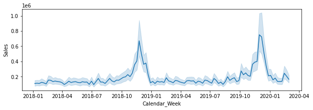
In particular, as seen above, we have data before covid and data during it, which should provide with a nice source of temporal environmental changes.

year_2020_began= datetime.datetime(2020, 1, 1)

training_data = data[data["Calendar_Week"] < year_2020_began]
test_data = data[data["Calendar_Week"] >= year_2020_began]

Logging these two sets in whylogs is a breeze.

whylogs v0

from whylogs import get_or_create_session

session = get_or_create_session()


profile_train= session.log_dataframe(training_data, 
                    dataset_timestamp=year_2020_began)
profile_test = session.log_dataframe(test_data, 
                    dataset_timestamp=datetime.datetime.utcnow())

whylogs v1

import whylogs as why
import datetime

profile_train= why.log(training_data).profile()
profile_train.set_dataset_timestamp(year_2020_began)

profile_test= why.log(test_data).profile()
profile_test.set_dataset_timestamp(datetime.datetime.utcnow())

In the background whylogs computes a myriad of statistics associated with each data type. Plotting the distribution for the "Overall views" features, shows a clear shift in these two sets.

We can quantify this shift, by using metrics like the Population Stability Index (PSI), Kolmogorov-Smirnov statistic (KS-test), Kullback-Lebler (KL) divergence (or other f-divergences), and histogram intersection. For example, given its popularity, we can compute the KL-divergence as a potential metric.

Next Steps

Check out notebook here for the example above.

What other shifts can you find ? Another powerful way to use these methods is to segment your data into specific groups. Allowing you to find, or alleviate potential sources bias into your model, collection method, or even in the inferred results themselves.