WhyLabs Algorithms
WhyLabs Algorithms
When monitoring data health, WhyLabs uses customizable algorithms at two different levels. First, WhyLabs uses an algorithm to compute the quantity to be monitored (e.g. distribution distance). WhyLabs then uses an algorithm to perform anomaly detection on these computed quantities. When computing distribution distances and performing anomaly detection, users have various options for the model baseline used for reference.
Anomaly Detection Algorithms
WhyLabs currently offers 3 customizable options for anomaly detection.
Standard Deviation (Default)
Used for monitoring of metrics that do not have seasonal patterns.
By default, WhyLabs detects anomalies of tracked metrics based on the number of standard deviations away from the mean. This tracked metric, along with its mean and standard deviation are computed using the baseline profile configured for a model.
For example, suppose a user chooses a reference window of 7 days for a particular model. Upon uploading a new profile, this profile’s distribution distance will be calculated against the aggregated distribution from profiles within the last 7 days. The mean and standard deviation of this distribution distance are calculated from the distribution distances computed in this way over the last 7 days.
If the distribution distance of the latest profile is more than some particular number of standard deviations away from the mean of these distribution distances, then an alert is generated. In the case of “learned” thresholds, this number of standard deviations is computed automatically using proprietary logic based on properties of the feature being monitored.
In the case of a single reference profile being selected instead of a rolling reference window, the square root of the mean is used as the standard deviation (standard deviation of a Poisson Distribution).
As an alternative to using an automatically computed number of standard deviations (learned threshold), users can set a fixed number of standard deviations that this threshold is computed from.
SARIMA
Used for metrics that have a seasonal pattern.
A Seasonal ARIMA (SARIMA) model can be used for anomaly detection in place of the default Standard Deviation algorithm. This algorithm is best for data which exhibits a seasonal pattern over a weekly, monthly, or quarterly cycle. The optimal seasonality can be determined via analysis or specified by the user. The default seasonality is 7 days.
The SARIMA algorithm is fit to data over some trailing window- 30 days by default. Users must have at least enough historical data to cover this trailing window for this algorithm to perform best.
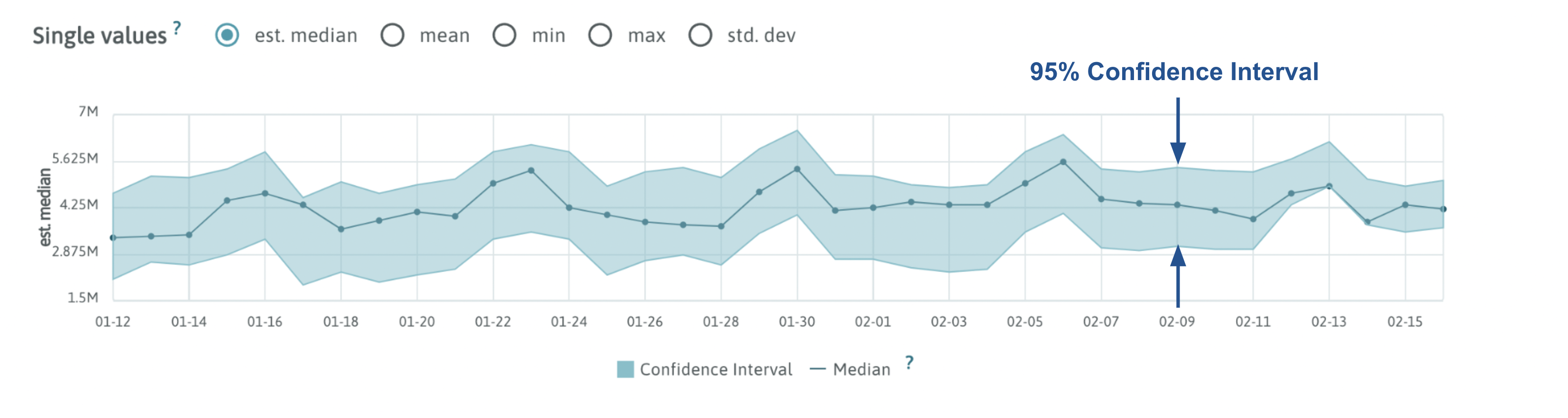
The SARIMA algorithm works by fitting itself to the data available within the selected trailing window. The output of this algorithm is a predicted value of the monitored metric along with a confidence interval surrounding it. If the observed value lies outside of this confidence interval, then an alert is generated.
When SARIMA or SARIMA + Standard Deviation algorithms are used for anomaly detection, the baseline chosen in the monitor settings is ignored for any monitors using either of these algorithms.
See this section on how the SARIMA algorithm works and how it's used for anomaly detection in WhyLabs.
Learn more about ARIMA and SARIMA.
SARIMA + Standard Deviation
Used for metrics that have a seasonal pattern with occasional, significant deviations from this seasonal pattern.
The SARIMA algorithm produces a confidence interval around the predicted value. If the incoming data undergoes significant deviations from its usual seasonal pattern, these confidence intervals can become large. During these deviations, the default standard deviation algorithm is superior, which does not assume seasonality.
The SARIMA + Standard Deviation algorithm is a modified version of the SARIMA algorithm designed to restrict these confidence intervals to 1 standard deviation from the predicted value in the event that the confidence interval becomes too wide due to data deviating from its seasonal pattern.
Distribution Distance Algorithms
WhyLabs’ Drift Monitors are based on distribution distances calculated from one of several algorithms. Each of these algorithms compares two distributions and computes a value representing how different the two distributions are.
Profiles generated by whylogs retain information necessary to reconstruct the approximate distributions as opposed to simply collecting certain descriptive statistics. This allows WhyLabs to utilize powerful algorithms for measuring distribution distances which would not be possible otherwise. Furthermore, the WhyLabs implementation of each distribution distance algorithm is compatible with both numeric (continuous and discrete) as well as categorical distributions.
Hellinger Distance
This is the default algorithm used to compute distribution distance. Hellinger distance is symmetric, is robust against missing values, and is easy to interpret. Two highly similar distributions will have a Hellinger distance close to 0 whereas two highly dissimilar distributions will have a Hellinger distance close to 1.
Range: 0 -1
Read more about the Hellinger Distance
Kolmogorov–Smirnov Test (KS Test)
Range: 0 - 1
The KS Test algorithm has similar performance to the Hellinger distance for the use case of detecting data drift. It should be noted that the output of the KS Test is a p-value rather than a distribution distance, which should be considered when interpreting this output.
Users will need to contact WhyLabs in order to have this algorithm enabled for measuring distribution distances.
Read more about KS Test
Kullback–Leibler Divergence (KL Divergence)
Range: 0 - ∞
The KL Divergence algorithm can also be used for measuring distribution distances. Despite the popularity of this algorithm, it’s typically less suitable for the data drift use case than the KS Test and Hellinger distance. This is partly due to its lack of symmetry and difficulty handling missing values.
Read more about KL Divergence
Other Algorithms
The Distribution Monitor, Missing Values Monitor, and Unique Values Monitor all use one of the two anomaly detection algorithms described previously. However, these algorithms do not apply to the Inferred Data Type Monitor and the Data Ingestion Monitor.
For the Inferred Data Type Monitor, WhyLabs generates an alert if the present data types differ from those contained in the baseline (single reference profile or reference window).
For the Data Ingestion Monitor, an alert will be sent if no profiles with timestamps within the last 2 days have been uploaded to the model.
Model Baselines
In order to compute distribution distances or detect anomalies, these algorithms need a baseline for reference. WhyLabs allows users to choose either a static reference profile or a sliding reference window.
Static Reference Profile
Users can choose a single reference profile which new profiles will be compared against. The distribution of this reference profile will be used when computing distribution distances with respect to new profiles and when detecting anomalies. Users typically choose one of the following as their static reference profile:
Training Set- Generating a static reference profile from a training set allows users to always know whether the data a model has been trained on is representative of the data which the model is making predictions on.
Ideal Dataset- Users may wish to generate a reference profile from an “ideal” dataset which meets the quality standards which are expected of incoming data.
Aggregated Dataset- Users can generate a profile from the combination of multiple batches of data over some span of time. This will help to incorporate organic fluctuations in the data which occur over short periods of time and don’t necessarily constitute drift. This is also a great option for small datasets.
Sliding Reference Window
Alternatively, users can choose a trailing reference window for their model baseline. This trailing window can be 7, 14, 21, or 28 days. This option is ideal for models which utilize online training or are frequently retrained.
The ideal length of the trailing window will depend on the details of the online training or retraining processes. For example, if a model using online training is able to learn quickly from new data, then a shorter trailing window will be sufficient. In any case, users are encouraged to experiment with monitor configuration to find the ideal signal to noise ratio in their alerts.
SARIMA Algorithm Deep Dive
The following provides a more in-depth description of how the SARIMA algorithm works and how it’s used for anomaly detection in WhyLabs.
SARIMA Overview
The SARIMA acronym stands for Seasonal Auto-Regressive Integrated Moving Average. SARIMA is a time-series forecasting model which combines properties from several different forecasting techniques.
Seasonal - Predictions are influenced by previous values and prediction errors which are offset by some number of seasonal cycles.
Auto-Regressive - Predictions are influenced by some configurable number of previous values immediately preceding the prediction.
Integrated - A differencing technique is performed some configurable number of times to arrive at an approximately stationary series (constant mean and variance) which can be more easily analyzed.
Moving Average - Predictions are influenced by the errors associated with some configurable number of previous predictions.
The SARIMA model takes the form of a linear expression with contributions from previous values in the series as well as contributions from prediction errors from previous timesteps.
This linear function is trained on some time series which has been transformed to be approximately stationary (constant mean and variance). This training process involves tuning the coefficients from this linear expression such that the squared error is minimized.
The form of this linear expression is determined by 7 hyper-parameters, commonly expressed as SARIMA(p,d,q)(P,D,Q)m.
The prediction errors of the trained model form a distribution which is used to calculate a 95% confidence interval surrounding the model’s prediction. WhyLabs utilizes this 95% confidence interval for anomaly detection and raises an alert for any observed values which fall outside of this confidence interval.
Non-Seasonal ARIMA Details
The (AR), (I) and (MA) parts of the model can be described by 3 parameters: p, d, q.
The d parameter relates to the “Integrated” part of SARIMA and its value determines how many times to transform raw data via “differencing”. This is done by redefining a series s to be equal to the difference between each consecutive time step:
Zt = st+1 - st
The goal is to transform the series into an approximately stationary series (constant mean, and variance) for easier analysis via forecasting methods. The image below shows the effect this transformation has on a non-stationary series:
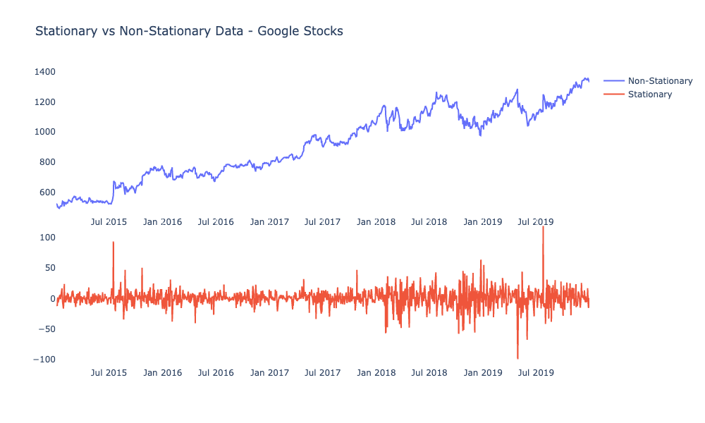
If the transformed series is not approximately stationary, this transformation can be repeated as many times as necessary. This transformation is analogous to taking a derivative. The SARIMA model is fit to this transformed series.
The p parameter relates to the “AR” part of SARIMA and its value determines how many recent values of the series are included as terms in our model. For example, if p=3, the 3 most recent values preceding our prediction will be included in our model as follows:
Zt = a0 + a1Zt-1 + a2Zt-2 + a3Zt-3
Here, ai represents the coefficients which are tuned by minimizing the squared error once combined with contributions from other parts of the SARIMA model.
The q parameter represents the “MA” part of the SARIMA model and its value determines how many recent predictions have their error values contributing to the model. For example, a q value of 2 would indicate that I will include errors from the past two predictions in my model. Each of these errors is also multiplied by some constant which is tuned by minimizing the squared error.
These 3 contributions are combined to form a non-seasonal ARIMA model. For example, training an ARIMA(3,2,2) model would entail the following.
- Transform the series via “differencing” two times (d parameter)
- Tune the coefficients of the following expression by minimizing the squared error.
Zt = a0 + a1Zt-1 + a2Zt-2 + a3Zt-3 + b1et-1 + b2et-2
The ai coefficients related to the “AR” portion of ARIMA (predictions are influenced by recent values). The bi coefficients relate to the “MA” part of ARIMA (new predictions will be influenced by recent prediction errors). Predictions undergo an inverse transformation to return to the original non-stationary series.
SARIMA Details
The “Seasonal” portion of SARIMA is configured via 4 other parameters- P, D, Q, m. The m parameter indicates how many timesteps constitute one seasonal cycle. The P, D, and Q parameters are seasonal analogues to the p, d, and q parameters.
For instance, setting p=2 and P=3 indicates that my model will include contributions from the 2 most recent values as well as contributions from the values which correspond to offsets of 1, 2, and 3 seasonal cycles from these values. The Q parameter operates similarly.
The D parameter serves a similar function as the d parameter, except that the series is transformed via a differencing against seasonal offsets rather than consecutive timestamps.
Implementing an SARIMA algorithm for anomaly detection in WhyLabs requires experimenting with the SARIMA hyperparameters to arrive at an optimal signal-to-noise ratio. The WhyLabs implementation of SARIMA requires at least 30 days of historical data in order for the algorithm to have a sufficient number of data points to effectively tune SARIMA’s coefficients and to generate a meaningful confidence interval for anomaly detection.

